转载: http://pandas.pydata.org/pandas-docs/stable/10min.html
翻译: shizhuolin@hotmail.com
10 Minutes to pandas
This is a short introduction to pandas, geared mainly for new users. You can see more complex recipes in the Cookbook
10分钟搞定pandas
这是关于pandas的简短介绍, 主要面向新用户. 可以参阅Cookbook了解更复杂的使用方法.
Customarily, we import as follows
习惯上,我们做以下导入
In [1]: import pandas as pd
In [2]: import numpy as np
In [3]: import matplotlib.pyplot as plt
Object Creation
创建对象
See the Data Structure Intro section 查看 数据结构简介 Creating a Series by passing a list of values, letting pandas create a default integer index
使用传递的值列表序列创建序列, 让pandas创建默认整数索引
In [4]: s = pd.Series([1,3,5,np.nan,6,8])
In [5]: s
Out[5]:
0     1
1     3
2     5
3   NaN
4     6
5     8
dtype: float64
Creating a DataFrame by passing a numpy array, with a datetime index and labeled columns.
使用传递的numpy数组创建数据帧,并使用日期索引和标记列.
In [6]: dates = pd.date_range('20130101',periods=6)
In [7]: dates
Out[7]:

[2013-01-01, ..., 2013-01-06]
Length: 6, Freq: D, Timezone: None

In [8]: df = pd.DataFrame(np.random.randn(6,4),index=dates,columns=list('ABCD'))
In [9]: df
Out[9]:
                   A         B         C         D
2013-01-01  0.469112 -0.282863 -1.509059 -1.135632
2013-01-02  1.212112 -0.173215  0.119209 -1.044236
2013-01-03 -0.861849 -2.104569 -0.494929  1.071804
2013-01-04  0.721555 -0.706771 -1.039575  0.271860
2013-01-05 -0.424972  0.567020  0.276232 -1.087401
2013-01-06 -0.673690  0.113648 -1.478427  0.524988
Creating a DataFrame by passing a dict of objects that can be converted to series-like.
使用传递的可转换序列的字典对象创建数据帧.
In [10]: df2 = pd.DataFrame({ 'A' : 1.,
   ....:                      'B' : pd.Timestamp('20130102'),
   ....:                      'C' : pd.Series(1,index=list(range(4)),dtype='float32'),
   ....:                      'D' : np.array([3] * 4,dtype='int32'),
   ....:                      'E' : pd.Categorical(["test","train","test","train"]),
   ....:                      'F' : 'foo' })
   ....:
In [11]: df2
Out[11]:
   A          B  C  D      E    F
0  1 2013-01-02  1  3   test  foo
1  1 2013-01-02  1  3  train  foo
2  1 2013-01-02  1  3   test  foo
3  1 2013-01-02  1  3  train  foo
In [12]: df2.dtypes
Out[12]:
A           float64
B    datetime64[ns]
C           float32
D             int32
E          category
F            object
dtype: object
If you’re using IPython, tab completion for column names (as well as public attributes) is automatically enabled. Here’s a subset of the attributes that will be completed:
如果你这个正在使用IPython,标签补全列名(以及公共属性)将自动启用。这里是将要完成的属性的子集:
In [13]: df2.
df2.A                  df2.boxplot
df2.abs                df2.C
df2.add                df2.clip
df2.add_prefix         df2.clip_lower
df2.add_suffix         df2.clip_upper
df2.align              df2.columns
df2.all                df2.combine
df2.any                df2.combineAdd
df2.append             df2.combine_first
df2.apply              df2.combineMult
df2.applymap           df2.compound
df2.as_blocks          df2.consolidate
df2.asfreq             df2.convert_objects
df2.as_matrix          df2.copy
df2.astype             df2.corr
df2.at                 df2.corrwith
df2.at_time            df2.count
df2.axes               df2.cov
df2.B                  df2.cummax
df2.between_time       df2.cummin
df2.bfill              df2.cumprod
df2.blocks             df2.cumsum
df2.bool               df2.D
As you can see, the columns A, B, C, and D are automatically tab completed. E is there as well; the rest of the attributes have been truncated for brevity.
如你所见, 列 A, B, C, 和 D 也是自动完成标签. E 也是可用的; 为了简便起见,后面的属性显示被截断.
Viewing Data
查看数据
See the Basics section
参阅基础部分
See the top & bottom rows of the frame
查看帧顶部和底部行
In [14]: df.head()
Out[14]:
                   A         B         C         D
2013-01-01  0.469112 -0.282863 -1.509059 -1.135632
2013-01-02  1.212112 -0.173215  0.119209 -1.044236
2013-01-03 -0.861849 -2.104569 -0.494929  1.071804
2013-01-04  0.721555 -0.706771 -1.039575  0.271860
2013-01-05 -0.424972  0.567020  0.276232 -1.087401

In [15]: df.tail(3)
Out[15]:
                   A         B         C         D
2013-01-04  0.721555 -0.706771 -1.039575  0.271860
2013-01-05 -0.424972  0.567020  0.276232 -1.087401
2013-01-06 -0.673690  0.113648 -1.478427  0.524988
Display the index,columns, and the underlying numpy data
显示索引,列,和底层numpy数据
In [16]: df.index
Out[16]:

[2013-01-01, ..., 2013-01-06]
Length: 6, Freq: D, Timezone: None

In [17]: df.columns
Out[17]: Index([u'A', u'B', u'C', u'D'], dtype='object')

In [18]: df.values
Out[18]:
array([[ 0.4691, -0.2829, -1.5091, -1.1356],
       [ 1.2121, -0.1732,  0.1192, -1.0442],
       [-0.8618, -2.1046, -0.4949,  1.0718],
       [ 0.7216, -0.7068, -1.0396,  0.2719],
       [-0.425 ,  0.567 ,  0.2762, -1.0874],
       [-0.6737,  0.1136, -1.4784,  0.525 ]])
Describe shows a quick statistic summary of your data
描述显示数据快速统计摘要
In [19]: df.describe()
Out[19]:
              A         B         C         D
count  6.000000  6.000000  6.000000  6.000000
mean   0.073711 -0.431125 -0.687758 -0.233103
std    0.843157  0.922818  0.779887  0.973118
min   -0.861849 -2.104569 -1.509059 -1.135632
25%   -0.611510 -0.600794 -1.368714 -1.076610
50%    0.022070 -0.228039 -0.767252 -0.386188
75%    0.658444  0.041933 -0.034326  0.461706
max    1.212112  0.567020  0.276232  1.071804
Transposing your data
转置数据
In [20]: df.T
Out[20]:
   2013-01-01  2013-01-02  2013-01-03  2013-01-04  2013-01-05  2013-01-06
A    0.469112    1.212112   -0.861849    0.721555   -0.424972   -0.673690
B   -0.282863   -0.173215   -2.104569   -0.706771    0.567020    0.113648
C   -1.509059    0.119209   -0.494929   -1.039575    0.276232   -1.478427
D   -1.135632   -1.044236    1.071804    0.271860   -1.087401    0.524988
Sorting by an axis
按轴排序
In [21]: df.sort_index(axis=1, ascending=False)
Out[21]:
                   D         C         B         A
2013-01-01 -1.135632 -1.509059 -0.282863  0.469112
2013-01-02 -1.044236  0.119209 -0.173215  1.212112
2013-01-03  1.071804 -0.494929 -2.104569 -0.861849
2013-01-04  0.271860 -1.039575 -0.706771  0.721555
2013-01-05 -1.087401  0.276232  0.567020 -0.424972
2013-01-06  0.524988 -1.478427  0.113648 -0.673690
Sorting by values
按值排序
In [22]: df.sort(columns='B')
Out[22]:
                   A         B         C         D
2013-01-03 -0.861849 -2.104569 -0.494929  1.071804
2013-01-04  0.721555 -0.706771 -1.039575  0.271860
2013-01-01  0.469112 -0.282863 -1.509059 -1.135632
2013-01-02  1.212112 -0.173215  0.119209 -1.044236
2013-01-06 -0.673690  0.113648 -1.478427  0.524988
2013-01-05 -0.424972  0.567020  0.276232 -1.087401
Selection
选择器
Note: While standard Python / Numpy expressions for selecting and setting are intuitive and come in handy for interactive work, for production code, we recommend the optimized pandas data access methods, .at, .iat, .loc, .iloc and .ix.
注释: 标准Python / Numpy表达式可以完成这些互动工作, 但在生产代码中, 我们推荐使用优化的pandas数据访问方法, .at, .iat, .loc, .iloc 和 .ix.
See the indexing documentation Indexing and Selecing Data and MultiIndex / Advanced Indexing
参阅索引文档 索引和选择数据 and 多索引/高级索引
Getting
读取
Selecting a single column, which yields a Series, equivalent to df.A
选择单列, 这会产生一个序列, 等价df.A
In [23]: df['A']
Out[23]:
2013-01-01    0.469112
2013-01-02    1.212112
2013-01-03   -0.861849
2013-01-04    0.721555
2013-01-05   -0.424972
2013-01-06   -0.673690
Freq: D, Name: A, dtype: float64
Selecting via [], which slices the rows.
使用[]选择行片断
In [24]: df[0:3]
Out[24]:
                   A         B         C         D
2013-01-01  0.469112 -0.282863 -1.509059 -1.135632
2013-01-02  1.212112 -0.173215  0.119209 -1.044236
2013-01-03 -0.861849 -2.104569 -0.494929  1.071804

In [25]: df['20130102':'20130104']
Out[25]:
                   A         B         C         D
2013-01-02  1.212112 -0.173215  0.119209 -1.044236
2013-01-03 -0.861849 -2.104569 -0.494929  1.071804
2013-01-04  0.721555 -0.706771 -1.039575  0.271860
Selection by Label
使用标签选择
See more in Selection by Label
更多信息请参阅按标签选择
For getting a cross section using a label
使用标签获取横截面
In [26]: df.loc[dates[0]]
Out[26]:
A    0.469112
B   -0.282863
C   -1.509059
D   -1.135632
Name: 2013-01-01 00:00:00, dtype: float64
Selecting on a multi-axis by label
使用标签选择多轴
In [27]: df.loc[:,['A','B']]
Out[27]:
                   A         B
2013-01-01  0.469112 -0.282863
2013-01-02  1.212112 -0.173215
2013-01-03 -0.861849 -2.104569
2013-01-04  0.721555 -0.706771
2013-01-05 -0.424972  0.567020
2013-01-06 -0.673690  0.113648
Showing label slicing, both endpoints are included
显示标签切片, 包含两个端点
In [28]: df.loc['20130102':'20130104',['A','B']]
Out[28]:
                   A         B
2013-01-02  1.212112 -0.173215
2013-01-03 -0.861849 -2.104569
2013-01-04  0.721555 -0.706771
Reduction in the dimensions of the returned object
降低返回对象维度
In [29]: df.loc['20130102',['A','B']]
Out[29]:
A    1.212112
B   -0.173215
Name: 2013-01-02 00:00:00, dtype: float64
For getting a scalar value
获取标量值
In [30]: df.loc[dates[0],'A']
Out[30]: 0.46911229990718628
For getting fast access to a scalar (equiv to the prior method)
快速访问并获取标量数据 (等价上面的方法)
In [31]: df.at[dates[0],'A']
Out[31]: 0.46911229990718628
Selection by Position
按位置选择
See more in Selection by Position
更多信息请参阅按位置参阅
Select via the position of the passed integers
传递整数选择位置
In [32]: df.iloc[3]
Out[32]:
A    0.721555
B   -0.706771
C   -1.039575
D    0.271860
Name: 2013-01-04 00:00:00, dtype: float64
By integer slices, acting similar to numpy/python
使用整数片断,效果类似numpy/python
In [33]: df.iloc[3:5,0:2]
Out[33]:
                   A         B
2013-01-04  0.721555 -0.706771
2013-01-05 -0.424972  0.567020
By lists of integer position locations, similar to the numpy/python style
使用整数偏移定位列表,效果类似 numpy/python 样式
In [34]: df.iloc[[1,2,4],[0,2]]
Out[34]:
                   A         C
2013-01-02  1.212112  0.119209
2013-01-03 -0.861849 -0.494929
2013-01-05 -0.424972  0.276232
For slicing rows explicitly
显式行切片
In [35]: df.iloc[1:3,:]
Out[35]:
                   A         B         C         D
2013-01-02  1.212112 -0.173215  0.119209 -1.044236
2013-01-03 -0.861849 -2.104569 -0.494929  1.071804
For slicing columns explicitly
显式列切片
In [36]: df.iloc[:,1:3]
Out[36]:
                   B         C
2013-01-01 -0.282863 -1.509059
2013-01-02 -0.173215  0.119209
2013-01-03 -2.104569 -0.494929
2013-01-04 -0.706771 -1.039575
2013-01-05  0.567020  0.276232
2013-01-06  0.113648 -1.478427
For getting a value explicitly
显式获取一个值
In [37]: df.iloc[1,1]
Out[37]: -0.17321464905330861
For getting fast access to a scalar (equiv to the prior method)
快速访问一个标量(等同上个方法)
In [38]: df.iat[1,1]
Out[38]: -0.17321464905330861
Boolean Indexing
布尔索引
Using a single column’s values to select data.
使用单个列的值选择数据.
In [39]: df[df.A > 0]
Out[39]:
                   A         B         C         D
2013-01-01  0.469112 -0.282863 -1.509059 -1.135632
2013-01-02  1.212112 -0.173215  0.119209 -1.044236
2013-01-04  0.721555 -0.706771 -1.039575  0.271860
A where operation for getting.
where 操作.
In [40]: df[df > 0]
Out[40]:
                   A         B         C         D
2013-01-01  0.469112       NaN       NaN       NaN
2013-01-02  1.212112       NaN  0.119209       NaN
2013-01-03       NaN       NaN       NaN  1.071804
2013-01-04  0.721555       NaN       NaN  0.271860
2013-01-05       NaN  0.567020  0.276232       NaN
2013-01-06       NaN  0.113648       NaN  0.524988
Using the isin() method for filtering:
使用 isin() 筛选:
In [41]: df2 = df.copy()
In [42]: df2['E']=['one', 'one','two','three','four','three']

In [43]: df2
Out[43]:
                   A         B         C         D      E
2013-01-01  0.469112 -0.282863 -1.509059 -1.135632    one
2013-01-02  1.212112 -0.173215  0.119209 -1.044236    one
2013-01-03 -0.861849 -2.104569 -0.494929  1.071804    two
2013-01-04  0.721555 -0.706771 -1.039575  0.271860  three
2013-01-05 -0.424972  0.567020  0.276232 -1.087401   four
2013-01-06 -0.673690  0.113648 -1.478427  0.524988  three

In [44]: df2[df2['E'].isin(['two','four'])]
Out[44]:
                   A         B         C         D     E
2013-01-03 -0.861849 -2.104569 -0.494929  1.071804   two
2013-01-05 -0.424972  0.567020  0.276232 -1.087401  four
Setting
赋值
Setting a new column automatically aligns the data by the indexes
赋值一个新列,通过索引自动对齐数据
In [45]: s1 = pd.Series([1,2,3,4,5,6],index=pd.date_range('20130102',periods=6))
In [46]: s1
Out[46]:
2013-01-02    1
2013-01-03    2
2013-01-04    3
2013-01-05    4
2013-01-06    5
2013-01-07    6
Freq: D, dtype: int64

In [47]: df['F'] = s1
Setting values by label
按标签赋值
In [48]: df.at[dates[0],'A'] = 0
Setting values by position
按位置赋值
In [49]: df.iat[0,1] = 0
Setting by assigning with a numpy array
通过numpy数组分配赋值
In [50]: df.loc[:,'D'] = np.array([5] * len(df))
The result of the prior setting operations
之前的操作结果
In [51]: df
Out[51]:
                   A         B         C  D   F
2013-01-01  0.000000  0.000000 -1.509059  5 NaN
2013-01-02  1.212112 -0.173215  0.119209  5   1
2013-01-03 -0.861849 -2.104569 -0.494929  5   2
2013-01-04  0.721555 -0.706771 -1.039575  5   3
2013-01-05 -0.424972  0.567020  0.276232  5   4
2013-01-06 -0.673690  0.113648 -1.478427  5   5
A where operation with setting.
where 操作赋值.
In [52]: df2 = df.copy()
In [53]: df2[df2 > 0] = -df2
In [54]: df2
Out[54]:
                   A         B         C  D   F
2013-01-01  0.000000  0.000000 -1.509059 -5 NaN
2013-01-02 -1.212112 -0.173215 -0.119209 -5  -1
2013-01-03 -0.861849 -2.104569 -0.494929 -5  -2
2013-01-04 -0.721555 -0.706771 -1.039575 -5  -3
2013-01-05 -0.424972 -0.567020 -0.276232 -5  -4
2013-01-06 -0.673690 -0.113648 -1.478427 -5  -5
Missing Data
丢失的数据
pandas primarily uses the value np.nan to represent missing data. It is by default not included in computations. See the Missing Data section
pandas主要使用np.nan替换丢失的数据. 默认情况下它并不包含在计算中. 请参阅 Missing Data section
Reindexing allows you to change/add/delete the index on a specified axis. This returns a copy of the data.
重建索引允许更改/添加/删除指定轴索引,并返回数据副本.
In [55]: df1 = df.reindex(index=dates[0:4],columns=list(df.columns) + ['E'])
In [56]: df1.loc[dates[0]:dates[1],'E'] = 1
In [57]: df1
Out[57]:
                   A         B         C  D   F   E
2013-01-01  0.000000  0.000000 -1.509059  5 NaN   1
2013-01-02  1.212112 -0.173215  0.119209  5   1   1
2013-01-03 -0.861849 -2.104569 -0.494929  5   2 NaN
2013-01-04  0.721555 -0.706771 -1.039575  5   3 NaN
To drop any rows that have missing data.
删除任何有丢失数据的行.
In [58]: df1.dropna(how='any')
Out[58]:
                   A         B         C  D  F  E
2013-01-02  1.212112 -0.173215  0.119209  5  1  1
Filling missing data
填充丢失数据
In [59]: df1.fillna(value=5)
Out[59]:
                   A         B         C  D  F  E
2013-01-01  0.000000  0.000000 -1.509059  5  5  1
2013-01-02  1.212112 -0.173215  0.119209  5  1  1
2013-01-03 -0.861849 -2.104569 -0.494929  5  2  5
2013-01-04  0.721555 -0.706771 -1.039575  5  3  5
To get the boolean mask where values are nan
获取值是否nan的布尔标记
In [60]: pd.isnull(df1)
Out[60]:
                A      B      C      D      F      E
2013-01-01  False  False  False  False   True  False
2013-01-02  False  False  False  False  False  False
2013-01-03  False  False  False  False  False   True
2013-01-04  False  False  False  False  False   True
Operations
运算
See the Basic section on Binary Ops
参阅二元运算基础
Stats
统计
Operations in general exclude missing data.
计算时一般不包括丢失的数据
Performing a descriptive statistic
执行描述性统计
In [61]: df.mean()
Out[61]:
A   -0.004474
B   -0.383981
C   -0.687758
D    5.000000
F    3.000000
dtype: float64
Same operation on the other axis
在其他轴做相同的运算
In [62]: df.mean(1)
Out[62]:
2013-01-01    0.872735
2013-01-02    1.431621
2013-01-03    0.707731
2013-01-04    1.395042
2013-01-05    1.883656
2013-01-06    1.592306
Freq: D, dtype: float64
Operating with objects that have different dimensionality and need alignment. In addition, pandas automatically broadcasts along the specified dimension.
用于运算的对象有不同的维度并需要对齐.除此之外,pandas会自动沿着指定维度计算.
In [63]: s = pd.Series([1,3,5,np.nan,6,8],index=dates).shift(2)
In [64]: s
Out[64]:
2013-01-01   NaN
2013-01-02   NaN
2013-01-03     1
2013-01-04     3
2013-01-05     5
2013-01-06   NaN
Freq: D, dtype: float64

In [65]: df.sub(s,axis='index')
Out[65]:
                   A         B         C   D   F
2013-01-01       NaN       NaN       NaN NaN NaN
2013-01-02       NaN       NaN       NaN NaN NaN
2013-01-03 -1.861849 -3.104569 -1.494929   4   1
2013-01-04 -2.278445 -3.706771 -4.039575   2   0
2013-01-05 -5.424972 -4.432980 -4.723768   0  -1
2013-01-06       NaN       NaN       NaN NaN NaN
Apply
Applying functions to the data
在数据上使用函数
In [66]: df.apply(np.cumsum)
Out[66]:
                   A         B         C   D   F
2013-01-01  0.000000  0.000000 -1.509059   5 NaN
2013-01-02  1.212112 -0.173215 -1.389850  10   1
2013-01-03  0.350263 -2.277784 -1.884779  15   3
2013-01-04  1.071818 -2.984555 -2.924354  20   6
2013-01-05  0.646846 -2.417535 -2.648122  25  10
2013-01-06 -0.026844 -2.303886 -4.126549  30  15

In [67]: df.apply(lambda x: x.max() - x.min())
Out[67]:
A    2.073961
B    2.671590
C    1.785291
D    0.000000
F    4.000000
dtype: float64
Histogramming
直方图
See more at Histogramming and Discretization
请参阅 直方图和离散化
In [68]: s = pd.Series(np.random.randint(0,7,size=10))
In [69]: s
Out[69]:
0    4
1    2
2    1
3    2
4    6
5    4
6    4
7    6
8    4
9    4
dtype: int32

In [70]: s.value_counts()
Out[70]:
4    5
6    2
2    2
1    1
dtype: int64
String Methods
字符串方法
Series is equipped with a set of string processing methods in the str attribute that make it easy to operate on each element of the array, as in the code snippet below. Note that pattern-matching in str generally uses regular expressions by default (and in some cases always uses them). See more at Vectorized String Methods.
序列可以使用一些字符串处理方法很轻易操作数据组中的每个元素,比如以下代码片断。 注意字符匹配方法默认情况下通常使用正则表达式(并且大多数时候都如此). 更多信息请参阅字符串向量方法.
In [71]: s = pd.Series(['A', 'B', 'C', 'Aaba', 'Baca', np.nan, 'CABA', 'dog', 'cat'])
In [72]: s.str.lower()
Out[72]:
0       a
1       b
2       c
3    aaba
4    baca
5     NaN
6    caba
7     dog
8     cat
dtype: object
Merge
合并
Concat
连接
pandas provides various facilities for easily combining together Series, DataFrame, and Panel objects with various kinds of set logic for the indexes and relational algebra functionality in the case of join / merge-type operations.
pandas提供各种工具以简便合并序列,数据桢,和组合对象, 在连接/合并类型操作中使用多种类型索引和相关数学函数.
See the Merging section
请参阅合并部分
Concatenating pandas objects together
把pandas对象连接到一起
In [73]: df = pd.DataFrame(np.random.randn(10, 4))
In [74]: df
Out[74]:
          0         1         2         3
0 -0.548702  1.467327 -1.015962 -0.483075
1  1.637550 -1.217659 -0.291519 -1.745505
2 -0.263952  0.991460 -0.919069  0.266046
3 -0.709661  1.669052  1.037882 -1.705775
4 -0.919854 -0.042379  1.247642 -0.009920
5  0.290213  0.495767  0.362949  1.548106
6 -1.131345 -0.089329  0.337863 -0.945867
7 -0.932132  1.956030  0.017587 -0.016692
8 -0.575247  0.254161 -1.143704  0.215897
9  1.193555 -0.077118 -0.408530 -0.862495

# break it into pieces
In [75]: pieces = [df[:3], df[3:7], df[7:]]
In [76]: pd.concat(pieces)
Out[76]:
          0         1         2         3
0 -0.548702  1.467327 -1.015962 -0.483075
1  1.637550 -1.217659 -0.291519 -1.745505
2 -0.263952  0.991460 -0.919069  0.266046
3 -0.709661  1.669052  1.037882 -1.705775
4 -0.919854 -0.042379  1.247642 -0.009920
5  0.290213  0.495767  0.362949  1.548106
6 -1.131345 -0.089329  0.337863 -0.945867
7 -0.932132  1.956030  0.017587 -0.016692
8 -0.575247  0.254161 -1.143704  0.215897
9  1.193555 -0.077118 -0.408530 -0.862495
Join
连接
SQL style merges. See the Database style joining
SQL样式合并. 请参阅 数据库style联接
In [77]: left = pd.DataFrame({'key': ['foo', 'foo'], 'lval': [1, 2]})
In [78]: right = pd.DataFrame({'key': ['foo', 'foo'], 'rval': [4, 5]})
In [79]: left
Out[79]:
   key  lval
0  foo     1
1  foo     2

In [80]: right
Out[80]:
   key  rval
0  foo     4
1  foo     5

In [81]: pd.merge(left, right, on='key')
Out[81]:
   key  lval  rval
0  foo     1     4
1  foo     1     5
2  foo     2     4
3  foo     2     5
Append
添加
Append rows to a dataframe. See the Appending
添加行到数据增. 参阅 添加
In [82]: df = pd.DataFrame(np.random.randn(8, 4), columns=['A','B','C','D'])
In [83]: df
Out[83]:
          A         B         C         D
0  1.346061  1.511763  1.627081 -0.990582
1 -0.441652  1.211526  0.268520  0.024580
2 -1.577585  0.396823 -0.105381 -0.532532
3  1.453749  1.208843 -0.080952 -0.264610
4 -0.727965 -0.589346  0.339969 -0.693205
5 -0.339355  0.593616  0.884345  1.591431
6  0.141809  0.220390  0.435589  0.192451
7 -0.096701  0.803351  1.715071 -0.708758

In [84]: s = df.iloc[3]
In [85]: df.append(s, ignore_index=True)
Out[85]:
          A         B         C         D
0  1.346061  1.511763  1.627081 -0.990582
1 -0.441652  1.211526  0.268520  0.024580
2 -1.577585  0.396823 -0.105381 -0.532532
3  1.453749  1.208843 -0.080952 -0.264610
4 -0.727965 -0.589346  0.339969 -0.693205
5 -0.339355  0.593616  0.884345  1.591431
6  0.141809  0.220390  0.435589  0.192451
7 -0.096701  0.803351  1.715071 -0.708758
8  1.453749  1.208843 -0.080952 -0.264610
Grouping
分组
By “group by” we are referring to a process involving one or more of the following steps
- Splitting the data into groups based on some criteria
- Applying a function to each group independently
- Combining the results into a data structure
对于“group by”指的是以下一个或多个处理
- 将数据按某些标准分割为不同的组
- 在每个独立组上应用函数
- 组合结果为一个数据结构
See the Grouping section
请参阅 分组部分
In [86]: df = pd.DataFrame({'A' : ['foo', 'bar', 'foo', 'bar',
   ....:                          'foo', 'bar', 'foo', 'foo'],
   ....:                    'B' : ['one', 'one', 'two', 'three',
   ....:                          'two', 'two', 'one', 'three'],
   ....:                    'C' : np.random.randn(8),
   ....:                    'D' : np.random.randn(8)})
   ....:
In [87]: df
Out[87]:
     A      B         C         D
0  foo    one -1.202872 -0.055224
1  bar    one -1.814470  2.395985
2  foo    two  1.018601  1.552825
3  bar  three -0.595447  0.166599
4  foo    two  1.395433  0.047609
5  bar    two -0.392670 -0.136473
6  foo    one  0.007207 -0.561757
7  foo  three  1.928123 -1.623033
Grouping and then applying a function sum to the resulting groups.
分组然后应用函数统计总和存放到结果组
In [88]: df.groupby('A').sum()
Out[88]:
            C        D
A
bar -2.802588  2.42611
foo  3.146492 -0.63958
Grouping by multiple columns forms a hierarchical index, which we then apply the function.
按多列分组为层次索引,然后应用函数
In [89]: df.groupby(['A','B']).sum()
Out[89]:
                  C         D
A   B
bar one   -1.814470  2.395985
    three -0.595447  0.166599
    two   -0.392670 -0.136473
foo one   -1.195665 -0.616981
    three  1.928123 -1.623033
    two    2.414034  1.600434
Reshaping
重塑
See the sections on Hierarchical Indexing and Reshaping.
请参阅章节 分层索引 和 重塑.
Stack
堆叠
In [90]: tuples = list(zip(*[['bar', 'bar', 'baz', 'baz',
   ....:                      'foo', 'foo', 'qux', 'qux'],
   ....:                     ['one', 'two', 'one', 'two',
   ....:                      'one', 'two', 'one', 'two']]))
   ....:
In [91]: index = pd.MultiIndex.from_tuples(tuples, names=['first', 'second'])
In [92]: df = pd.DataFrame(np.random.randn(8, 2), index=index, columns=['A', 'B'])
In [93]: df2 = df[:4]
In [94]: df2
Out[94]:
                     A         B
first second
bar   one     0.029399 -0.542108
      two     0.282696 -0.087302
baz   one    -1.575170  1.771208
      two     0.816482  1.100230
The stack function “compresses” a level in the DataFrame’s columns.
堆叠 函数 “压缩” 数据桢的列一个级别.
In [95]: stacked = df2.stack()
In [96]: stacked
Out[96]:
first  second
bar    one     A    0.029399
               B   -0.542108
       two     A    0.282696
               B   -0.087302
baz    one     A   -1.575170
               B    1.771208
       two     A    0.816482
               B    1.100230
dtype: float64
With a “stacked” DataFrame or Series (having a MultiIndex as the index), the inverse operation of stack is unstack, which by default unstacks the last level:
被“堆叠”数据桢或序列(有多个索引作为索引), 其堆叠的反向操作是未堆栈, 上面的数据默认反堆叠到上一级别:
In [97]: stacked.unstack()
Out[97]:
                     A         B
first second
bar   one     0.029399 -0.542108
      two     0.282696 -0.087302
baz   one    -1.575170  1.771208
      two     0.816482  1.100230

In [98]: stacked.unstack(1)
Out[98]:
second        one       two
first
bar   A  0.029399  0.282696
      B -0.542108 -0.087302
baz   A -1.575170  0.816482
      B  1.771208  1.100230

In [99]: stacked.unstack(0)
Out[99]:
first          bar       baz
second
one    A  0.029399 -1.575170
       B -0.542108  1.771208
two    A  0.282696  0.816482
       B -0.087302  1.100230
Pivot Tables
数据透视表
See the section on Pivot Tables.
查看数据透视表.
In [100]: df = pd.DataFrame({'A' : ['one', 'one', 'two', 'three'] * 3,
   .....:                    'B' : ['A', 'B', 'C'] * 4,
   .....:                    'C' : ['foo', 'foo', 'foo', 'bar', 'bar', 'bar'] * 2,
   .....:                    'D' : np.random.randn(12),
   .....:                    'E' : np.random.randn(12)})
   .....:
In [101]: df
Out[101]:
        A  B    C         D         E
0     one  A  foo  1.418757 -0.179666
1     one  B  foo -1.879024  1.291836
2     two  C  foo  0.536826 -0.009614
3   three  A  bar  1.006160  0.392149
4     one  B  bar -0.029716  0.264599
5     one  C  bar -1.146178 -0.057409
6     two  A  foo  0.100900 -1.425638
7   three  B  foo -1.035018  1.024098
8     one  C  foo  0.314665 -0.106062
9     one  A  bar -0.773723  1.824375
10    two  B  bar -1.170653  0.595974
11  three  C  bar  0.648740  1.167115
We can produce pivot tables from this data very easily:
我们可以从此数据非常容易的产生数据透视表:
In [102]: pd.pivot_table(df, values='D', index=['A', 'B'], columns=['C'])
Out[102]:
C             bar       foo
A     B
one   A -0.773723  1.418757
      B -0.029716 -1.879024
      C -1.146178  0.314665
three A  1.006160       NaN
      B       NaN -1.035018
      C  0.648740       NaN
two   A       NaN  0.100900
      B -1.170653       NaN
      C       NaN  0.536826
Time Series
时间序列
pandas has simple, powerful, and efficient functionality for performing resampling operations during frequency conversion (e.g., converting secondly data into 5-minutely data). This is extremely common in, but not limited to, financial applications. See the Time Series section
pandas有易用,强大且高效的函数用于高频数据重采样转换操作(例如,转换秒数据到5分钟数据), 这是很普遍的情况,但并不局限于金融应用, 请参阅时间序列章节
In [103]: rng = pd.date_range('1/1/2012', periods=100, freq='S')
In [104]: ts = pd.Series(np.random.randint(0, 500, len(rng)), index=rng)
In [105]: ts.resample('5Min', how='sum')
Out[105]:
2012-01-01    25083
Freq: 5T, dtype: int32
Time zone representation
时区表示
In [106]: rng = pd.date_range('3/6/2012 00:00', periods=5, freq='D')
In [107]: ts = pd.Series(np.random.randn(len(rng)), rng)
In [108]: ts
Out[108]:
2012-03-06    0.464000
2012-03-07    0.227371
2012-03-08   -0.496922
2012-03-09    0.306389
2012-03-10   -2.290613
Freq: D, dtype: float64

In [109]: ts_utc = ts.tz_localize('UTC')
In [110]: ts_utc
Out[110]:
2012-03-06 00:00:00+00:00    0.464000
2012-03-07 00:00:00+00:00    0.227371
2012-03-08 00:00:00+00:00   -0.496922
2012-03-09 00:00:00+00:00    0.306389
2012-03-10 00:00:00+00:00   -2.290613
Freq: D, dtype: float64
Convert to another time zone
转换到其它时区
In [111]: ts_utc.tz_convert('US/Eastern')
Out[111]:
2012-03-05 19:00:00-05:00    0.464000
2012-03-06 19:00:00-05:00    0.227371
2012-03-07 19:00:00-05:00   -0.496922
2012-03-08 19:00:00-05:00    0.306389
2012-03-09 19:00:00-05:00   -2.290613
Freq: D, dtype: float64
Converting between time span representations
转换不同的时间跨度
In [112]: rng = pd.date_range('1/1/2012', periods=5, freq='M')
In [113]: ts = pd.Series(np.random.randn(len(rng)), index=rng)
In [114]: ts
Out[114]:
2012-01-31   -1.134623
2012-02-29   -1.561819
2012-03-31   -0.260838
2012-04-30    0.281957
2012-05-31    1.523962
Freq: M, dtype: float64

In [115]: ps = ts.to_period()
In [116]: ps
Out[116]:
2012-01   -1.134623
2012-02   -1.561819
2012-03   -0.260838
2012-04    0.281957
2012-05    1.523962
Freq: M, dtype: float64

In [117]: ps.to_timestamp()
Out[117]:
2012-01-01   -1.134623
2012-02-01   -1.561819
2012-03-01   -0.260838
2012-04-01    0.281957
2012-05-01    1.523962
Freq: MS, dtype: float64
Converting between period and timestamp enables some convenient arithmetic functions to be used. In the following example, we convert a quarterly frequency with year ending in November to 9am of the end of the month following the quarter end:
转换时段并且使用一些运算函数, 下例中, 我们转换年报11月到季度结束每日上午9点数据
In [118]: prng = pd.period_range('1990Q1', '2000Q4', freq='Q-NOV')
In [119]: ts = pd.Series(np.random.randn(len(prng)), prng)
In [120]: ts.index = (prng.asfreq('M', 'e') + 1).asfreq('H', 's') + 9
In [121]: ts.head()
Out[121]:
1990-03-01 09:00   -0.902937
1990-06-01 09:00    0.068159
1990-09-01 09:00   -0.057873
1990-12-01 09:00   -0.368204
1991-03-01 09:00   -1.144073
Freq: H, dtype: float64
Categoricals
分类
Since version 0.15, pandas can include categorical data in a DataFrame. For full docs, see the categorical introduction and the API documentation.
自版本0.15起, pandas可以在数据桢中包含分类. 完整的文档, 请查看分类介绍 and the API文档.
In [122]: df = pd.DataFrame({"id":[1,2,3,4,5,6], "raw_grade":['a', 'b', 'b', 'a', 'a', 'e']})
Convert the raw grades to a categorical data type.
转换原始类别为分类数据类型.
In [123]: df["grade"] = df["raw_grade"].astype("category")
In [124]: df["grade"]
Out[124]:
0    a
1    b
2    b
3    a
4    a
5    e
Name: grade, dtype: category
Categories (3, object): [a, b, e]
Rename the categories to more meaningful names (assigning to Series.cat.categories is inplace!)
重命令分类为更有意义的名称 (分配到Series.cat.categories对应位置!)
In [125]: df["grade"].cat.categories = ["very good", "good", "very bad"]
Reorder the categories and simultaneously add the missing categories (methods under Series .cat return a new Series per default).
Reorder the categories and simultaneously add the missing categories (methods under Series .cat return a new Series per default).
重排顺分类,同时添加缺少的分类(序列 .cat方法下返回新默认序列)
In [126]: df["grade"] = df["grade"].cat.set_categories(["very bad", "bad", "medium", "good", "very good"])
In [127]: df["grade"]
Out[127]:
0    very good
1         good
2         good
3    very good
4    very good
5     very bad
Name: grade, dtype: category
Categories (5, object): [very bad, bad, medium, good, very good]
Sorting is per order in the categories, not lexical order.
排列分类中的顺序,不是按词汇排列.
In [128]: df.sort("grade")
Out[128]:
   id raw_grade      grade
5   6         e   very bad
1   2         b       good
2   3         b       good
0   1         a  very good
3   4         a  very good
4   5         a  very good
Grouping by a categorical column shows also empty categories.
类别列分组,并且也显示空类别.
In [129]: df.groupby("grade").size()
Out[129]:
grade
very bad      1
bad         NaN
medium      NaN
good          2
very good     3
dtype: float64
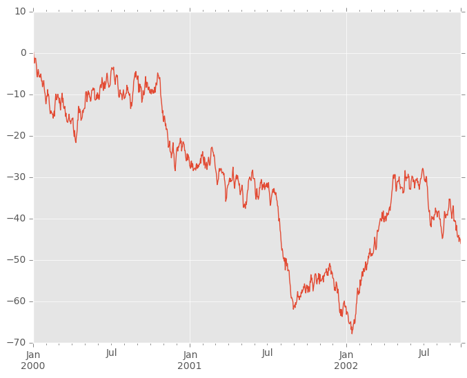
Plotting
绘图
In [130]: ts = pd.Series(np.random.randn(1000), index=pd.date_range('1/1/2000', periods=1000))
In [131]: ts = ts.cumsum()
In [132]: ts.plot()
Out[132]:
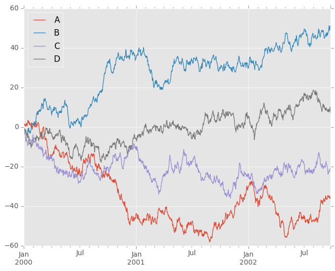
On DataFrame, plot is a convenience to plot all of the columns with labels:
在数据桢中,可以很方便的绘制带标签列:
In [133]: df = pd.DataFrame(np.random.randn(1000, 4), index=ts.index,
   .....:                   columns=['A', 'B', 'C', 'D'])
   .....:
In [134]: df = df.cumsum()
In [135]: plt.figure(); df.plot(); plt.legend(loc='best')
Out[135]:
Getting Data In/Out
获取数据输入/输出
CSV
In [136]: df.to_csv('foo.csv')
Reading from a csv file
读取csv文件
In [137]: pd.read_csv('foo.csv')
Out[137]:
     Unnamed: 0          A          B         C          D
0    2000-01-01   0.266457  -0.399641 -0.219582   1.186860
1    2000-01-02  -1.170732  -0.345873  1.653061  -0.282953
2    2000-01-03  -1.734933   0.530468  2.060811  -0.515536
3    2000-01-04  -1.555121   1.452620  0.239859  -1.156896
4    2000-01-05   0.578117   0.511371  0.103552  -2.428202
5    2000-01-06   0.478344   0.449933 -0.741620  -1.962409
6    2000-01-07   1.235339  -0.091757 -1.543861  -1.084753
..          ...        ...        ...       ...        ...
993  2002-09-20 -10.628548  -9.153563 -7.883146  28.313940
994  2002-09-21 -10.390377  -8.727491 -6.399645  30.914107
995  2002-09-22  -8.985362  -8.485624 -4.669462  31.367740
996  2002-09-23  -9.558560  -8.781216 -4.499815  30.518439
997  2002-09-24  -9.902058  -9.340490 -4.386639  30.105593
998  2002-09-25 -10.216020  -9.480682 -3.933802  29.758560
999  2002-09-26 -11.856774 -10.671012 -3.216025  29.369368

[1000 rows x 5 columns]
HDF5
Reading and writing to HDFStores
读写HDF存储
Writing to a HDF5 Store
写入HDF5存储
In [138]: df.to_hdf('foo.h5','df')
Reading from a HDF5 Store
读取HDF5存储
In [139]: pd.read_hdf('foo.h5','df')
Out[139]:
                    A          B         C          D
2000-01-01   0.266457  -0.399641 -0.219582   1.186860
2000-01-02  -1.170732  -0.345873  1.653061  -0.282953
2000-01-03  -1.734933   0.530468  2.060811  -0.515536
2000-01-04  -1.555121   1.452620  0.239859  -1.156896
2000-01-05   0.578117   0.511371  0.103552  -2.428202
2000-01-06   0.478344   0.449933 -0.741620  -1.962409
2000-01-07   1.235339  -0.091757 -1.543861  -1.084753
...               ...        ...       ...        ...
2002-09-20 -10.628548  -9.153563 -7.883146  28.313940
2002-09-21 -10.390377  -8.727491 -6.399645  30.914107
2002-09-22  -8.985362  -8.485624 -4.669462  31.367740
2002-09-23  -9.558560  -8.781216 -4.499815  30.518439
2002-09-24  -9.902058  -9.340490 -4.386639  30.105593
2002-09-25 -10.216020  -9.480682 -3.933802  29.758560
2002-09-26 -11.856774 -10.671012 -3.216025  29.369368

[1000 rows x 4 columns]
Excel
Reading and writing to MS Excel
读写MS Excel
Writing to an excel file
写入excel文件
In [140]: df.to_excel('foo.xlsx', sheet_name='Sheet1')
Reading from an excel file
读取excel文件
In [141]: pd.read_excel('foo.xlsx', 'Sheet1', index_col=None, na_values=['NA'])
Out[141]:
                    A          B         C          D
2000-01-01   0.266457  -0.399641 -0.219582   1.186860
2000-01-02  -1.170732  -0.345873  1.653061  -0.282953
2000-01-03  -1.734933   0.530468  2.060811  -0.515536
2000-01-04  -1.555121   1.452620  0.239859  -1.156896
2000-01-05   0.578117   0.511371  0.103552  -2.428202
2000-01-06   0.478344   0.449933 -0.741620  -1.962409
2000-01-07   1.235339  -0.091757 -1.543861  -1.084753
...               ...        ...       ...        ...
2002-09-20 -10.628548  -9.153563 -7.883146  28.313940
2002-09-21 -10.390377  -8.727491 -6.399645  30.914107
2002-09-22  -8.985362  -8.485624 -4.669462  31.367740
2002-09-23  -9.558560  -8.781216 -4.499815  30.518439
2002-09-24  -9.902058  -9.340490 -4.386639  30.105593
2002-09-25 -10.216020  -9.480682 -3.933802  29.758560
2002-09-26 -11.856774 -10.671012 -3.216025  29.369368

[1000 rows x 4 columns]
Gotchas
陷阱
If you are trying an operation and you see an exception like:
如果尝试这样操作可能会看到像这样的异常:
>>> if pd.Series([False, True, False]):
    print("I was true")
Traceback
    ...
ValueError: The truth value of an array is ambiguous. Use a.empty, a.any() or a.all().
See Comparisons for an explanation and what to do.
查看对照获取解释和怎么做的帮助
也可以查看陷阱.
mark!支持卓林哥!
群QQ群QQ群