Fit Data with a Neural Network

转载:http://cn.mathworks.com/help/nnet/gs/fit-data-with-a-neural-network.html

Neural networks are good at fitting functions. In fact, there is proof that a fairly simple neural network can fit any practical function.

Suppose, for instance, that you have data from a housing application. You want to design a network that can predict the value of a house (in $1000s), given 13 pieces of geographical and real estate information. You have a total of 506 example homes for which you have those 13 items of data and their associated market values.

You can solve this problem in two ways:

Use a graphical user interface, nftool, as described in Using the Neural Network Fitting Tool.
Use command-line functions, as described in Using Command-Line Functions.

It is generally best to start with the GUI, and then to use the GUI to automatically generate command-line scripts. Before using either method, first define the problem by selecting a data set. Each GUI has access to many sample data sets that you can use to experiment with the toolbox (see Neural Network Toolbox Sample Data Sets). If you have a specific problem that you want to solve, you can load your own data into the workspace. The next section describes the data format.

Defining a Problem

To define a fitting problem for the toolbox, arrange a set of Q input vectors as columns in a matrix. Then, arrange another set of Q target vectors (the correct output vectors for each of the input vectors) into a second matrix (see “Data Structures” for a detailed description of data formatting for static and time series data). For example, you can define the fitting problem for a Boolean AND gate with four sets of two-element input vectors and one-element targets as follows:

inputs = [0 1 0 1; 0 0 1 1];
targets = [0 0 0 1];

The next section shows how to train a network to fit a data set, using the neural network fitting tool GUI, nftool. This example uses the housing data set provided with the toolbox.

Using the Neural Network Fitting Tool

Open the Neural Network Start GUI with this command:
```
nnstart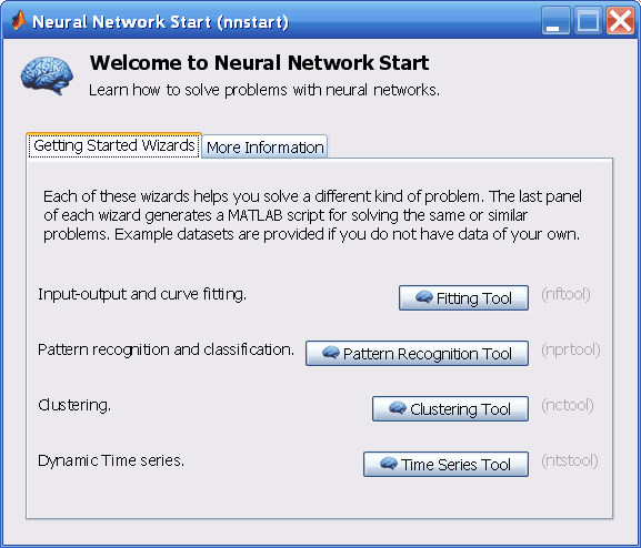
```
Click Fitting Tool to open the Neural Network Fitting Tool. (You can also use the command nftool.)
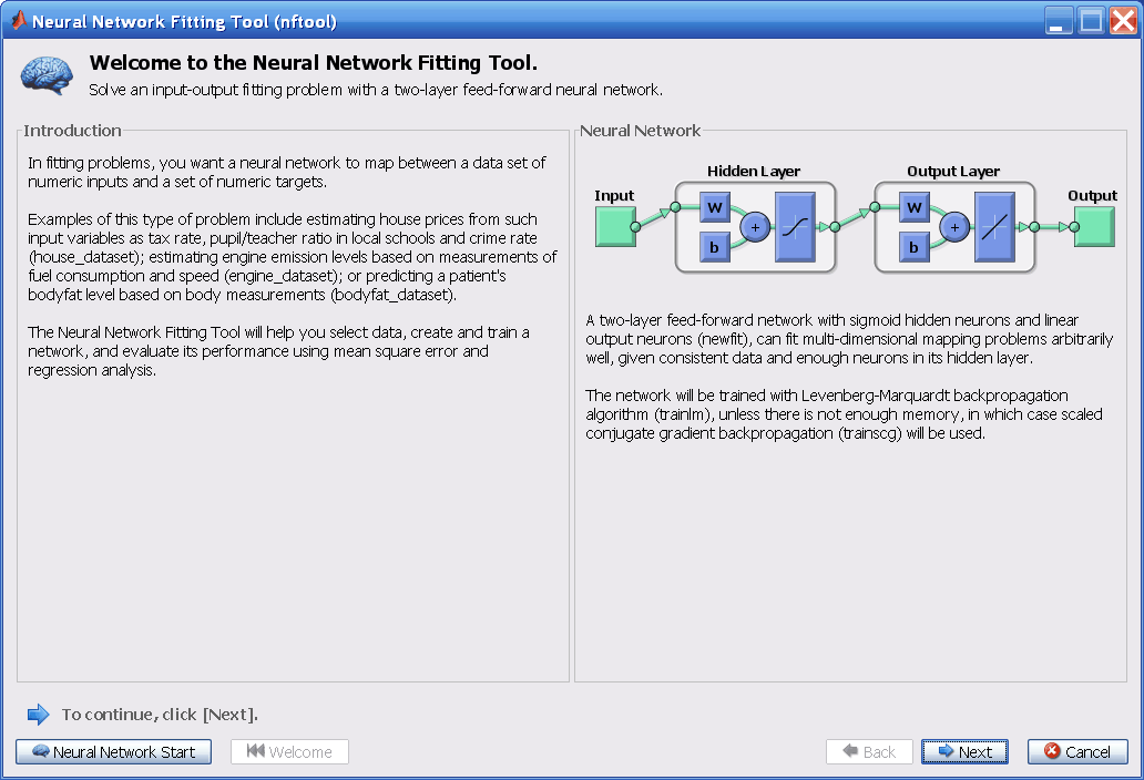
Click Next to proceed.
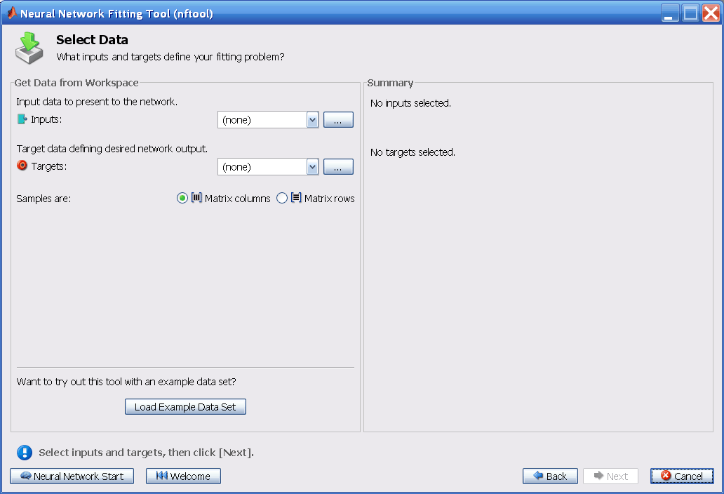
Click Load Example Data Set in the Select Data window. The Fitting Data Set Chooser window opens.

Note Use the Inputs and Targets options in the Select Data window when you need to load data from the MATLAB® workspace.
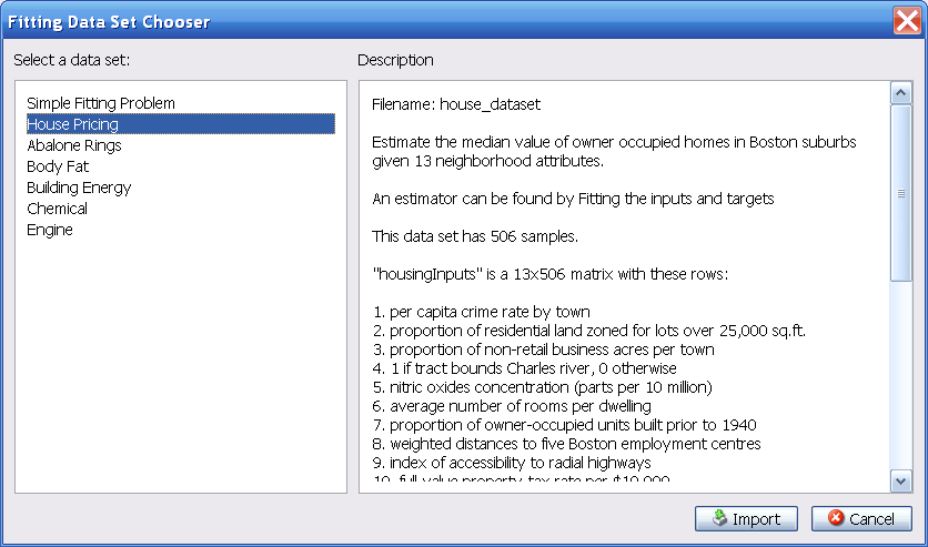
Select House Pricing, and click Import. This returns you to the Select Data window.
Click Next to display the Validation and Test Data window, shown in the following figure.
The validation and test data sets are each set to 15% of the original data.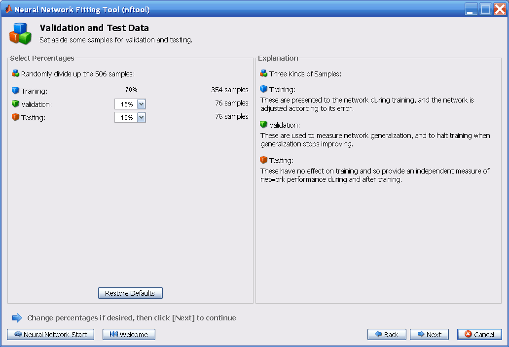 With these settings, the input vectors and target vectors will be randomly divided into three sets as follows:
- 70% will be used for training.
- 15% will be used to validate that the network is generalizing and to stop training before overfitting.
- The last 15% will be used as a completely independent test of network generalization.
(See “Dividing the Data” for more discussion of the data division process.)
Click Next.
The standard network that is used for function fitting is a two-layer feedforward network, with a sigmoid transfer function in the hidden layer and a linear transfer function in the output layer. The default number of hidden neurons is set to 10. You might want to increase this number later, if the network training performance is poor.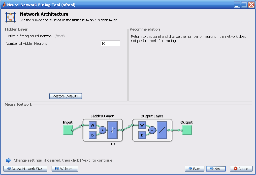
Click Next.
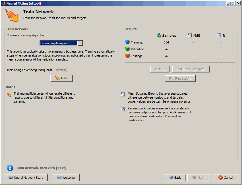
Select a training algorithm, then click Train.. Levenberg-Marquardt (trainlm) is recommended for most problems, but for some noisy and small problems Bayesian Regularization (trainbr) can take longer but obtain a better solution. For large problems, however, Scaled Conjugate Gradient (trainscg) is recommended as it uses gradient calculations which are more memory efficient than the Jacobian calculations the other two algorithms use. This example uses the default Levenberg-Marquardt.
The training continued until the validation error failed to decrease for six iterations (validation stop).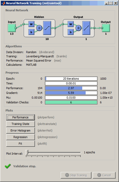
Under Plots, click Regression. This is used to validate the network performance.
The following regression plots display the network outputs with respect to targets for training, validation, and test sets. For a perfect fit, the data should fall along a 45 degree line, where the network outputs are equal to the targets. For this problem, the fit is reasonably good for all data sets, with R values in each case of 0.93 or above. If even more accurate results were required, you could retrain the network by clicking Retrain in nftool. This will change the initial weights and biases of the network, and may produce an improved network after retraining. Other options are provided on the following pane.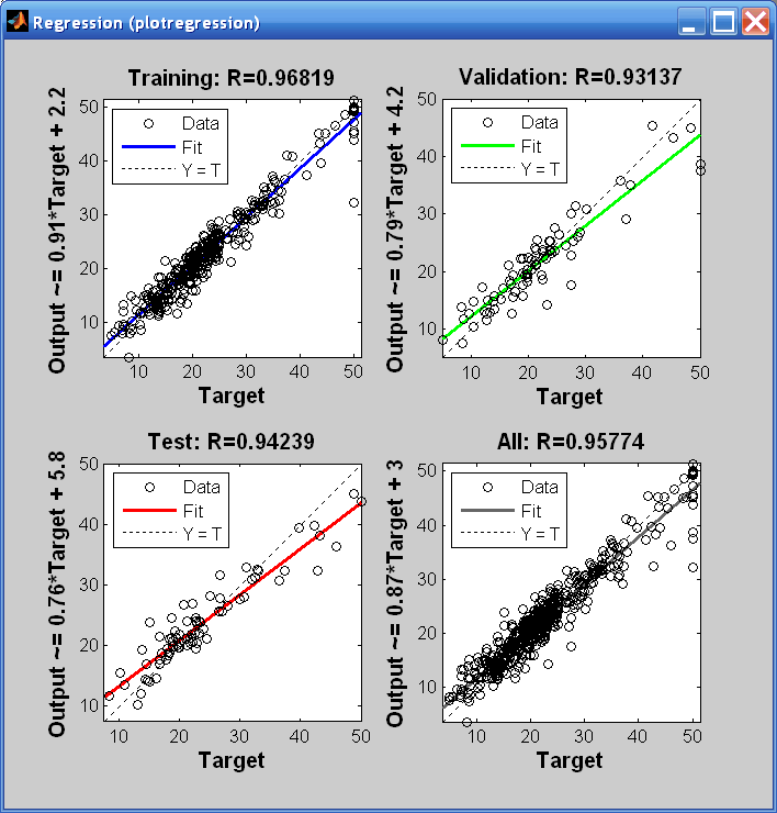
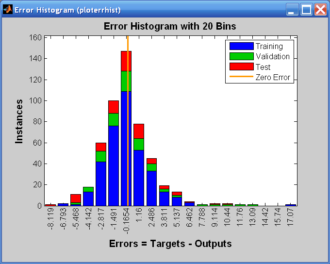
View the error histogram to obtain additional verification of network performance. Under the Plots pane, click Error Histogram. The blue bars represent training data, the green bars represent validation data, and the red bars represent testing data. The histogram can give you an indication of outliers, which are data points where the fit is significantly worse than the majority of data. In this case, you can see that while most errors fall between -5 and 5, there is a training point with an error of 17 and validation points with errors of 12 and 13. These outliers are also visible on the testing regression plot. The first corresponds to the point with a target of 50 and output near 33. It is a good idea to check the outliers to determine if the data is bad, or if those data points are different than the rest of the data set. If the outliers are valid data points, but are unlike the rest of the data, then the network is extrapolating for these points. You should collect more data that looks like the outlier points, and retrain the network.
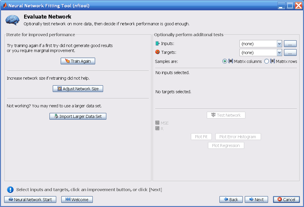
Click Next in the Neural Network Fitting Tool to evaluate the network. At this point, you can test the network against new data.
If you are dissatisfied with the network’s performance on the original or new data, you can do one of the following:
- Train it again.
- Increase the number of neurons.
- Get a larger training data set.
If the performance on the training set is good, but the test set performance is significantly worse, which could indicate overfitting, then reducing the number of neurons can improve your results. If training performance is poor, then you may want to increase the number of neurons.
If you are satisfied with the network performance, click Next.
Use this panel to generate a MATLAB function or Simulink® diagram for simulating your neural network. You can use the generated code or diagram to better understand how your neural network computes outputs from inputs, or deploy the network with MATLAB Compiler™ tools and other MATLAB code generation tools.
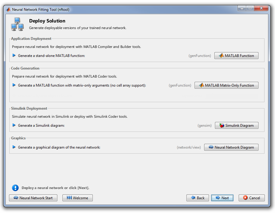
Use the buttons on this screen to generate scripts or to save your results.
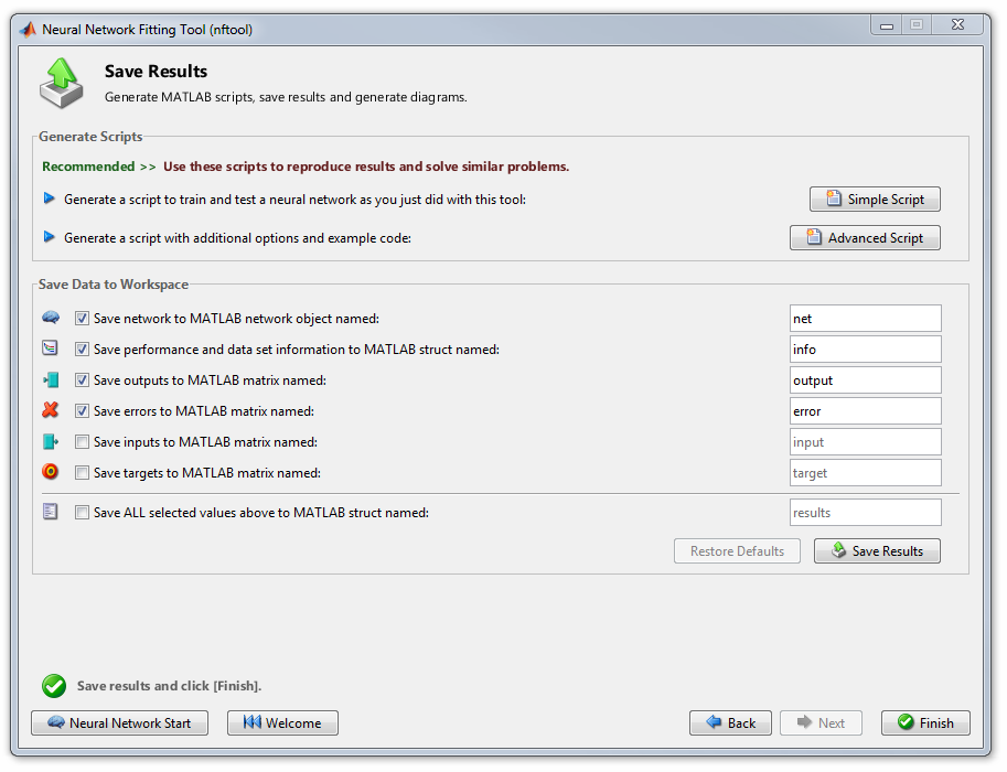
- You can click Simple Script or Advanced Script to create MATLAB code that can be used to reproduce all of the previous steps from the command line. Creating MATLAB code can be helpful if you want to learn how to use the command-line functionality of the toolbox to customize the training process. In Using Command-Line Functions, you will investigate the generated scripts in more detail.
- You can also have the network saved as net in the workspace. You can perform additional tests on it or put it to work on new inputs.
When you have created the MATLAB code and saved your results, click Finish.

Using Command-Line Functions

The easiest way to learn how to use the command-line functionality of the toolbox is to generate scripts from the GUIs, and then modify them to customize the network training. As an example, look at the simple script that was created at step 14 of the previous section.

% Solve an Input-Output Fitting problem with a Neural Network
% Script generated by NFTOOL
%
% This script assumes these variables are defined:
%
%   houseInputs - input data.
%   houseTargets - target data.
 
inputs = houseInputs;
targets = houseTargets;
 
% Create a Fitting Network
hiddenLayerSize = 10;
net = fitnet(hiddenLayerSize);

% Set up Division of Data for Training, Validation, Testing
net.divideParam.trainRatio = 70/100;
net.divideParam.valRatio = 15/100;
net.divideParam.testRatio = 15/100;
 
% Train the Network
[net,tr] = train(net,inputs,targets);
 
% Test the Network
outputs = net(inputs);
errors = gsubtract(outputs,targets);
performance = perform(net,targets,outputs)
 
% View the Network
view(net)
 
% Plots
% Uncomment these lines to enable various plots.
%figure, plotperform(tr)
%figure, plottrainstate(tr)
%figure, plotfit(targets,outputs)
%figure, plotregression(targets,outputs)
%figure, ploterrhist(errors)

You can save the script, and then run it from the command line to reproduce the results of the previous GUI session. You can also edit the script to customize the training process. In this case, follow each step in the script.

The script assumes that the input vectors and target vectors are already loaded into the workspace. If the data are not loaded, you can load them as follows:
```
load house_dataset
inputs = houseInputs;
targets = houseTargets;
```
This data set is one of the sample data sets that is part of the toolbox (see Neural Network Toolbox Sample Data Sets). You can see a list of all available data sets by entering the command help nndatasets. The load command also allows you to load the variables from any of these data sets using your own variable names. For example, the command
```
[inputs,targets] = house_dataset;
```
will load the housing inputs into the array inputs and the housing targets into the array targets.
Create a network. The default network for function fitting (or regression) problems, fitnet, is a feedforward network with the default tan-sigmoid transfer function in the hidden layer and linear transfer function in the output layer. You assigned ten neurons (somewhat arbitrary) to the one hidden layer in the previous section. The network has one output neuron, because there is only one target value associated with each input vector.
```
hiddenLayerSize = 10;
net = fitnet(hiddenLayerSize);
```
Note More neurons require more computation, and they have a tendency to overfit the data when the number is set too high, but they allow the network to solve more complicated problems. More layers require more computation, but their use might result in the network solving complex problems more efficiently. To use more than one hidden layer, enter the hidden layer sizes as elements of an array in the fitnet command.
Set up the division of data.
```
net.divideParam.trainRatio = 70/100;
net.divideParam.valRatio = 15/100;
net.divideParam.testRatio = 15/100;
```
With these settings, the input vectors and target vectors will be randomly divided, with 70% used for training, 15% for validation and 15% for testing. (See “Dividing the Data” for more discussion of the data division process.)
Train the network. The network uses the default Levenberg-Marquardt algorithm (trainlm) for training. For problems in which Levenberg-Marquardt does not produce as accurate results as desired, or for large data problems, consider setting the network training function to Bayesian Regularization (trainbr) or Scaled Conjugate Gradient (trainscg), respectively, with either
```
net.trainFcn = 'trainbr';
net.trainFcn = 'trainscg';
```
To train the network, enter:
```
[net,tr] = train(net,inputs,targets);
```
During training, the following training window opens. This window displays training progress and allows you to interrupt training at any point by clicking Stop Training.

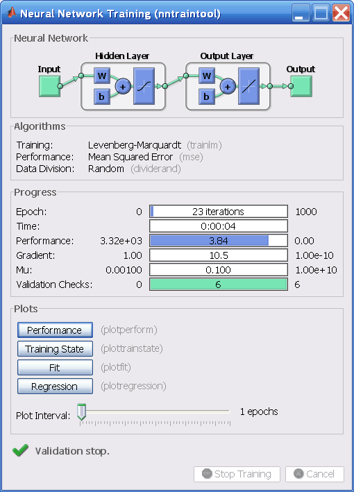
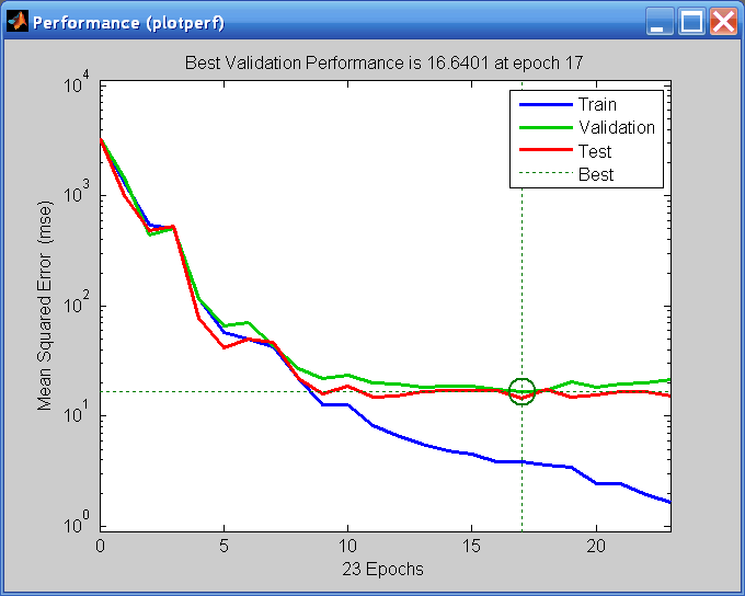
This training stopped when the validation error increased for six iterations, which occurred at iteration 23. If you click Performance in the training window, a plot of the training errors, validation errors, and test errors appears, as shown in the following figure. In this example, the result is reasonable because of the following considerations:
- The final mean-square error is small.
- The test set error and the validation set error have similar characteristics.
- No significant overfitting has occurred by iteration 17 (where the best validation performance occurs).
Test the network. After the network has been trained, you can use it to compute the network outputs. The following code calculates the network outputs, errors and overall performance.
```
outputs = net(inputs);
errors = gsubtract(targets,outputs);
performance = perform(net,targets,outputs)
```
```
performance =

    6.0023
```
It is also possible to calculate the network performance only on the test set, by using the testing indices, which are located in the training record. (See Analyze Neural Network Performance After Training for a full description of the training record.)
```
tInd = tr.testInd;
tstOutputs = net(inputs(tInd));
tstPerform = perform(net,targets(tInd),tstOutputs)
```
```
tstPerform =

   1.5700e+03
```
Perform some analysis of the network response. If you click Regression in the training window, you can perform a linear regression between the network outputs and the corresponding targets.
The following figure shows the results.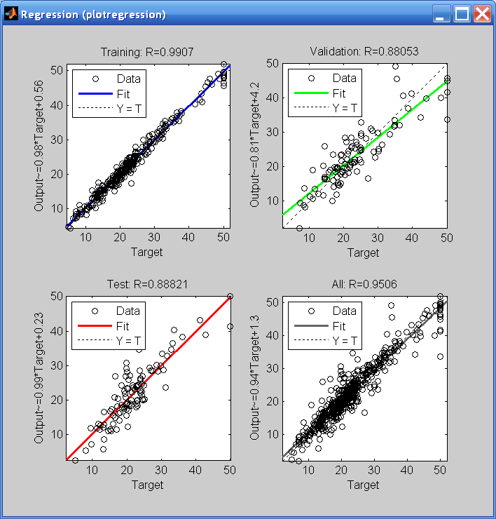

The output tracks the targets very well for training, testing, and validation, and the R-value is over 0.95 for the total response. If even more accurate results were required, you could try any of these approaches:
- Reset the initial network weights and biases to new values with init and train again (see “Initializing Weights” (init)).
- Increase the number of hidden neurons.
- Increase the number of training vectors.
- Increase the number of input values, if more relevant information is available.
- Try a different training algorithm (see “Training Algorithms“).
In this case, the network response is satisfactory, and you can now put the network to use on new inputs.
View the network diagram.
```
view(net)
```
To get more experience in command-line operations, try some of these tasks:
- During training, open a plot window (such as the regression plot), and watch it animate.
- Plot from the command line with functions such as plotfit, plotregression, plottrainstate and plotperform. (For more information on using these functions, see their reference pages.)
Also, see the advanced script for more options, when training from the command line.

Each time a neural network is trained, can result in a different solution due to different initial weight and bias values and different divisions of data into training, validation, and test sets. As a result, different neural networks trained on the same problem can give different outputs for the same input. To ensure that a neural network of good accuracy has been found, retrain several times.

There are several other techniques for improving upon initial solutions if higher accuracy is desired. For more information, see Improve Neural Network Generalization and Avoid Overfitting.

Shi Zhuolin's Blog

This guy is lazy, leaving nothing left.

Fit Data with a Neural Network